Tutorial
This page is a complete walkthrough of cool_maps. A runnable version of the same material lives in
notebooks/tutorial.ipynb in
the source repository.
Everything for making maps lives in cool_maps.plot, conventionally imported as cplt:
import cool_maps.plot as cplt

# Which mapping engines are importable in this environment, and which is active?
cplt.available_engines()   # ('cartopy', 'basemap') or ('cartopy',)
cplt.get_engine()          # 'cartopy'
If available_engines() only shows ('cartopy',), that’s fine – Cartopy is the default and only
required engine. Basemap is optional (see Choosing between Cartopy and Basemap below); everything in this tutorial up through
Overlaying your own data works identically either way.
Your first map
Every map starts with an extent: the bounding box you want to plot, as
(lon_min, lon_max, lat_min, lat_max). The only required argument to cplt.create() is extent
– everything else has a sensible default: tan land, blue ocean, black coastlines, automatically spaced
ticks, and rivers/lakes/state and country borders drawn in for you:
# Gulf of Mexico
extent = [-99, -79, 18, 31]

fig, ax = cplt.create(extent, gridlines=True)
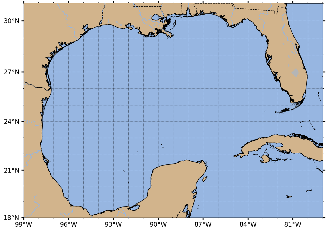
create() returns (fig, ax) when it builds a new figure for you (as above), or just ax if you
pass in an existing axes with ax=. ax is a normal matplotlib axes – you can call any standard
matplotlib method on it (ax.set_title(...), ax.legend(), etc.) in addition to the
cool_maps-specific behavior described below.
By default, create() expands your extent outward by padding=0.25 degrees on every side before
using it, so ticks (and any data you plot right at the edge of your bounding box) don’t land exactly on
the border of the map. Pass a single number to change the amount, a (lon_padding, lat_padding) pair
for asymmetric padding, or padding=0 to use extent exactly as given:
cplt.create(extent, padding=0)                # no padding -- old behavior
cplt.create(extent, padding=0.5)              # half a degree on every side
cplt.create(extent, padding=(1, 0.25))        # 1 degree lon, 0.25 degree lat
The padded extent is what’s actually used to build the axes, so it also determines the tick positions
(cplt.add_ticks()) and, when bathymetry=True, the bounding box that’s downloaded.
Projections
Pass proj= to pick a map projection. cool_maps accepts either a plain string (works under any
engine) or, if you’re using Cartopy, a real cartopy.crs object for full control.
Supported projection strings: "platecarree", "mercator" (the default), "lambertcylindrical",
"mill", "orthographic", "lambertconformal", "stereographic", "azimuthequidistant":
cplt.create(extent, proj="lambertcylindrical")
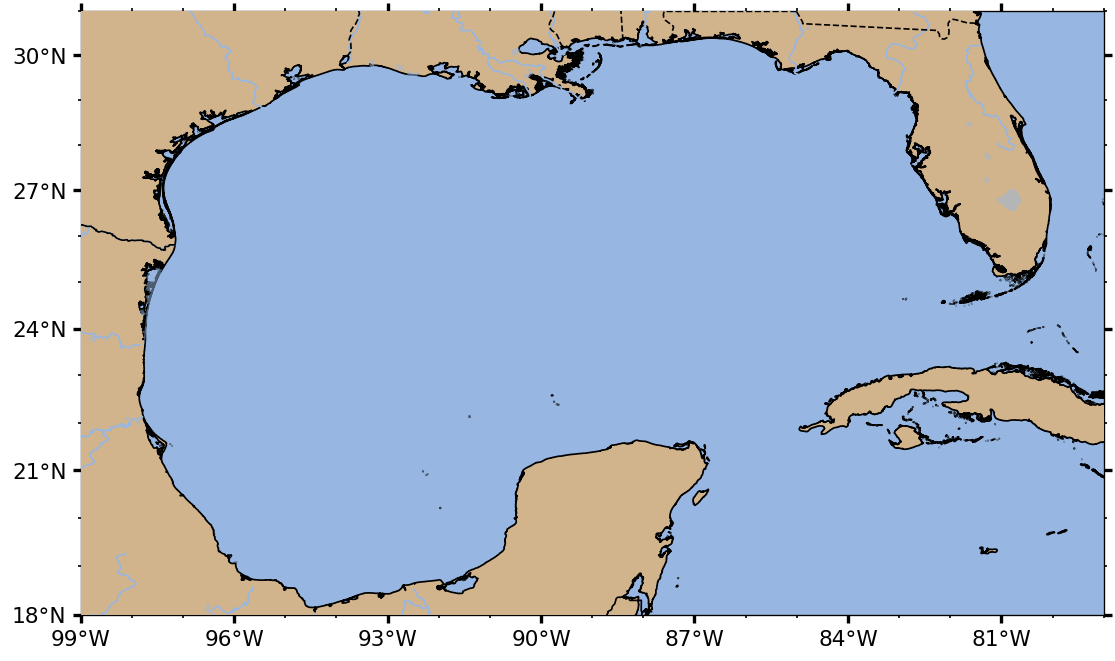
If you’re using the Cartopy engine, you can also pass a real CRS object for full control over projection parameters that the shared string form doesn’t expose:
import cartopy.crs as ccrs

cplt.create(extent, proj=ccrs.AlbersEqualArea(central_longitude=-89))
Coastline resolution
coast= controls how detailed the coastline/land polygons are. Higher resolution looks better for
regional maps but is slower to render.
coast= |
Use for |
|---|---|
full |
Regional/coastal maps needing maximum detail (the default) |
high |
Regional maps where “full” is too slow |
mid |
Basin-scale maps |
low |
Ocean-basin or global maps |
crude |
Quick previews; omits rivers/state borders |
Colors
Three keywords control the map’s color palette, independent of engine or projection:
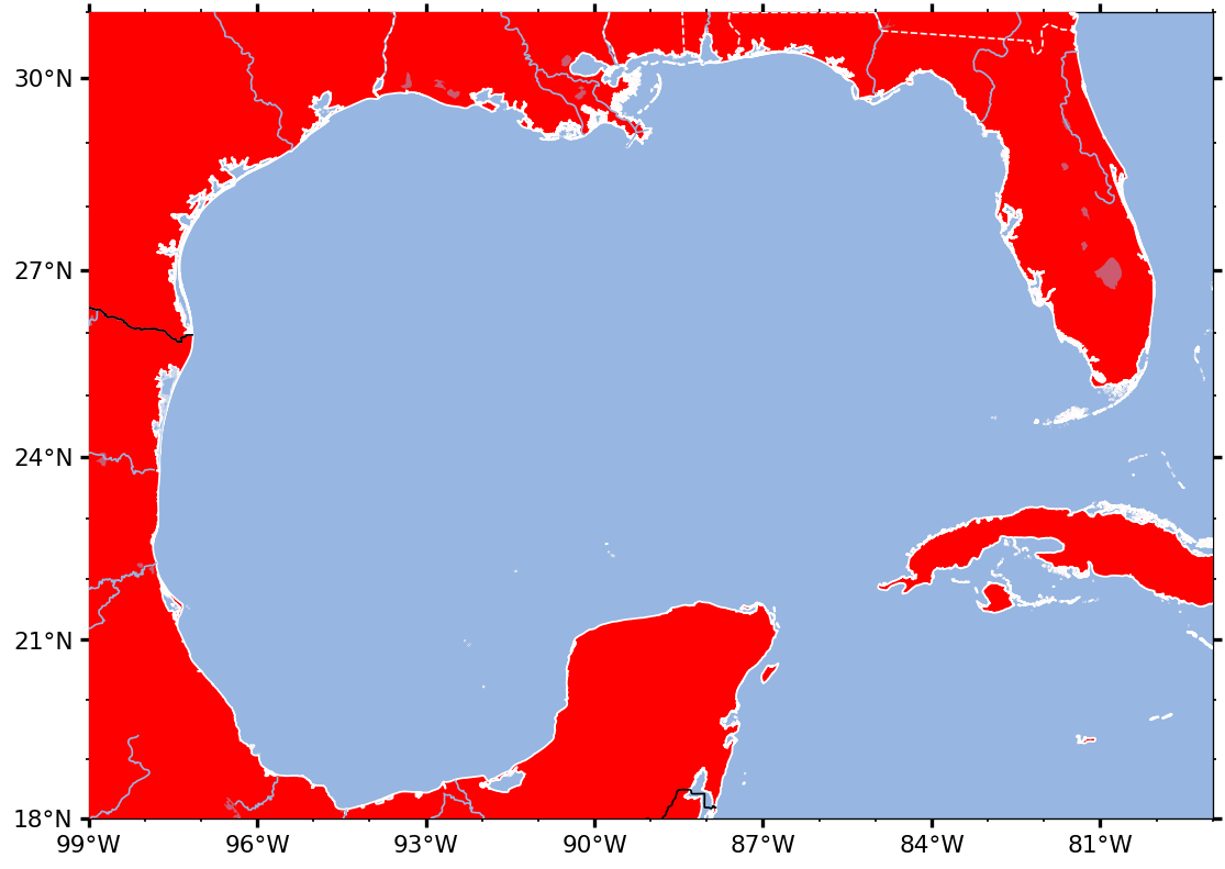
landcolor– fill color for land (default"tan")oceancolor– fill color for water (default: a Cartopy-style ocean blue)edgecolor– coastline/border line color (default"black")
cplt.create(extent, proj="mercator", landcolor="red", edgecolor="white")
Ticks and gridlines
ticks=True(default) computes nicely spaced tick positions from your extent, labeled in degrees-minutes-seconds by default.decimal_degrees=Trueswitches the labels to plain decimal degrees.gridlines=Trueoverlays a dashed grid at the tick positions.tick_label_left/_right/_bottom/_topcontrol which sides carry labels.
Bathymetry
Set bathymetry=True to download bathymetry data (GEBCO, via the Rutgers ERDDAP/THREDDS server) for
your extent and overlay it. isobaths= picks which depths to contour, and bathymetry_method= picks
the rendering style:
bathymetry_method |
Description |
|---|---|
contour (default) |
Black isobath lines at each depth in |
shadedcontour |
Isobaths shaded from light to dark grey with depth, plus a legend |
banded |
Discrete depth bands filled with explicit colors, or a built-in default for the 3-band case; plus the usual isobath lines/labels and a legend |
blues |
Continuous depth shading (Blues colormap); land masked out |
blues_log |
Same, with a log-transformed depth scale |
topo |
Continuous depth shading (cmocean |
topofull |
Same as |
Bathymetry downloads are cached to disk after the first call, so repeated calls for the same extent are
fast. Very large extents are automatically split into 10-degree tiles before being requested from the
server (Rutgers THREDDS rejects single OpenDAP requests that are too large), then stitched back together
– this is transparent when going through create(). If you call get_bathymetry() directly, pass
chunk_size= (in degrees) to change the tile size, or chunk_size=None to disable tiling:
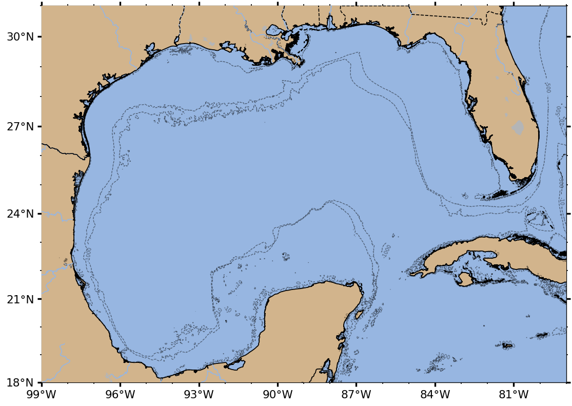
cplt.create(extent, proj="mercator", bathymetry=True)
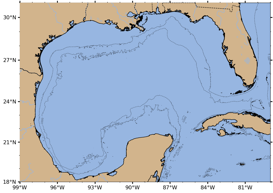
cplt.create(extent, proj="mercator", bathymetry=True, isobaths=(-1000, -500, -10))
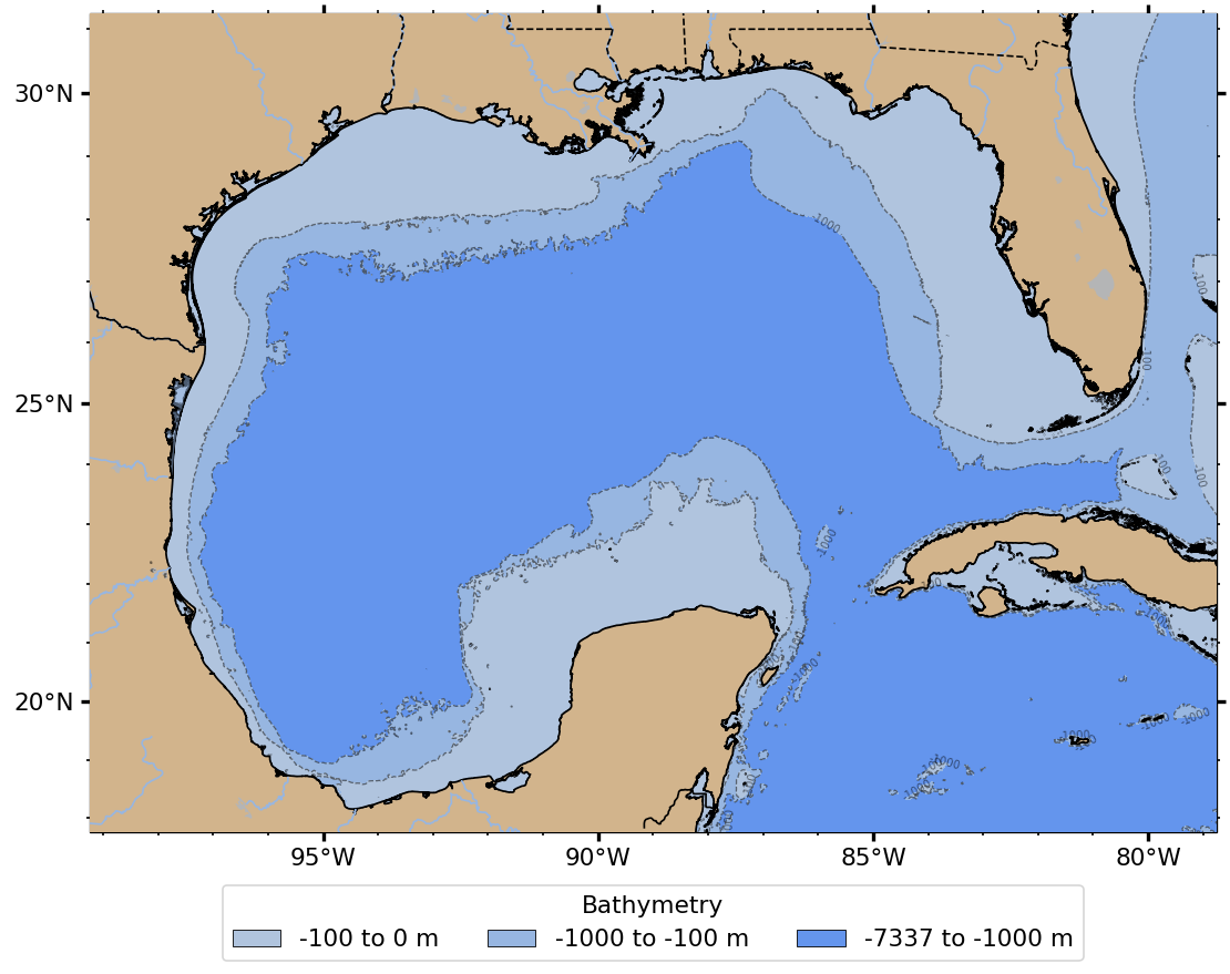
banded needs one more color than the number of isobaths, ordered from deepest to shallowest (the
extra color is for the band from the data’s minimum elevation down to the shallowest level). The default
isobaths=(-1000, -100) produces exactly 3 bands, which has a built-in default color scheme (deep,
cfeature.COLORS["water"] for the middle band, shallow) – so it works with no bathymetry_colors=
at all:
cplt.create(extent, bathymetry=True, bathymetry_method="banded")
Pass bathymetry_colors= to customize it (any other isobaths length requires this, since there’s
no default to guess from):
cplt.create(
    extent, bathymetry=True, bathymetry_method="banded",
    isobaths=(-3000, -1000, -100),
    bathymetry_colors=["navy", "cornflowerblue", "lightblue", "lightsteelblue"],
)
Overlaying your own data
ax (returned by create()) accepts plain longitude/latitude data directly on the usual matplotlib
plotting methods: scatter, plot, contour, contourf, pcolormesh, quiver, and
fill. cool_maps takes care of the coordinate-system detail behind the scenes (Cartopy needs a
transform= keyword; Basemap needs latlon=True) so you never have to think about it – the same
call works regardless of which engine built the axes:
fig, ax = cplt.create(extent, coast="low")
sc = ax.scatter(lons, lats, c=sst_anom, cmap="RdBu_r", vmin=-3, vmax=3, s=20, zorder=200)
cplt.add_colorbar(ax, sc, label="SST anomaly (°C)")
For point markers specifically, cplt.add_marker() is a thin convenience wrapper around the same
idea:
cplt.add_marker(ax, lon=-87.5, lat=25.5, marker="*", color="gold", s=300, edgecolor="black")
cplt.add_currents() plots a quiver field from an xarray.Dataset containing u/v velocity
components on lon/lat (or x/y) coordinates:
cplt.add_currents(ax, ds, coarsen=3)
If your map already has a legend (e.g. from bathymetry_method="shadedcontour" or "banded") and you
want a second one for your own overlaid data, use cplt.add_legend() in place of ax.legend() –
a plain second ax.legend() call replaces the first legend outright. add_legend() preserves
whatever legend is already there (handling a couple of non-obvious matplotlib details involved in doing
that correctly) before creating the new one, so you can call it repeatedly to build up any number of
legends on the same axes:
sc = ax.scatter(argo_lon, argo_lat, marker="^", color="red", label="Argo surfacing")
cplt.add_legend(ax, handles=[sc], loc="upper left")
See notebooks/banded_bathymetry_example.ipynb for a complete walkthrough, including how to
reposition each legend independently.
Choosing between Cartopy and Basemap
Everything above works identically regardless of which engine is active. Cartopy is the default and the
only required dependency; Basemap is optional (conda install -c conda-forge basemap basemap-data-hires,
or pip install cool_maps[basemap]).
There are three ways to pick an engine:
Per call, with
engine=– doesn’t touch the global default:cplt.create(extent, engine="basemap")
Globally, for the rest of the session:
cplt.set_engine("basemap")
cplt.create(extent)   # uses basemap
cplt.set_engine("cartopy")  # restore the default
Via the
COOL_MAPS_ENGINEenvironment variable, set before you importcool_maps.plot:COOL_MAPS_ENGINE=basemap python my_script.py
One more thing worth knowing: the axes returned by create() remembers which engine built it, so you
never need to pass engine= to add_features() / add_bathymetry() / add_currents() /
add_ticks() yourself – it’s inferred from the axes automatically. You only need engine= when you
want to override what the axes would otherwise infer.
When switching engines you can keep using the same Cartopy CRS objects in calls such as
cplt.create(..., proj=ccrs.Mercator()) – the Basemap backend will translate a handful of common
projections automatically. If a CRS cannot be converted, pass the Basemap projection name or keyword
dictionary instead (for example proj={'projection': 'lcc', 'lon_0': -74, 'lat_0': 39}).
Building a map piece by piece
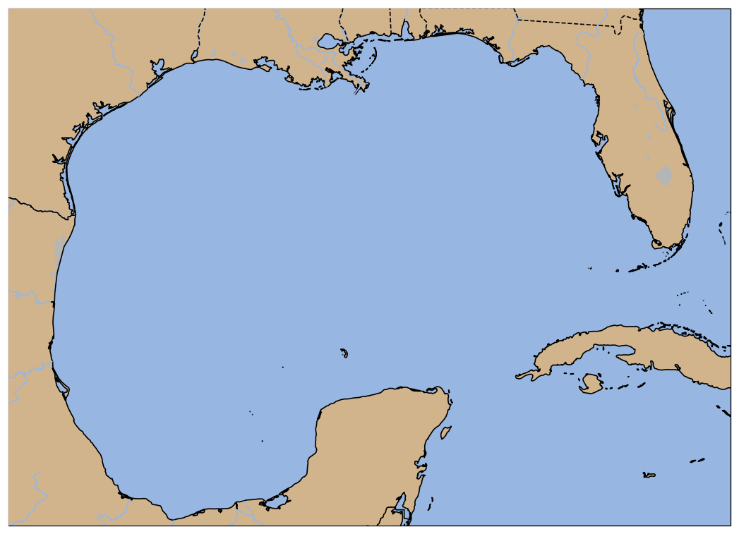
Setting features=False gives you a bare axes in the chosen projection, with none of the land/ocean/
border styling applied – useful if you want full control, or want to apply the default styling with
different colors/resolution after the fact via cplt.add_features() (rather than reaching for
engine-specific methods like Cartopy’s ax.add_feature(), which won’t work if the axes turns out to be
a Basemap axes):
fig, ax = cplt.create(extent, features=False, ticks=False)

# add_features() is the engine-agnostic way to add the land/ocean/border styling back in,
# with whatever customization you want -- it works no matter which engine built `ax`.
cplt.add_features(ax, landcolor="tan", oceancolor=None, edgecolor="black", coast="high", zorder=0.1)
Saving your figures
cplt.export_fig() is a thin wrapper around plt.savefig() that trims the whitespace around the
plot:
cplt.export_fig(save_path, "my_map.png")
cplt.save_fig() / cplt.load_fig() can pickle a whole figure for later reuse, but note that a
figure’s engine-specific instrumentation (and, for Basemap, the attached Basemap object) is not
guaranteed to survive a pickle round-trip – treat a reloaded figure’s axes as plain matplotlib axes
rather than a fully re-instrumented cool_maps axes.
Where to go next
Full API reference: cool_maps, or
help(cplt)from a Python session.notebooks/dual_backend_demo.ipynbin the source repository – a deeper dive into Cartopy/Basemap parity, including a performance comparison between the two engines.notebooks/engine_demo.ipynb– a minimal smoke test that both engines render without errors.